
From K-NN, HNSW to Product Quantization: Approximate Nearest Neighbor Search for vector search engines
Why do you need ANN? | Background
Elastic Search, Faiss and etc. all adopted their own approximate nearest neighbor search algorithms to deal with vector search among the huge scale of corpus. During my near research for my final-year project (FYP), which is to develop a production-level distributed search engine, I have looked into vector search, inverted index and Learning-to-Rank, for my main and the most used features — searching .
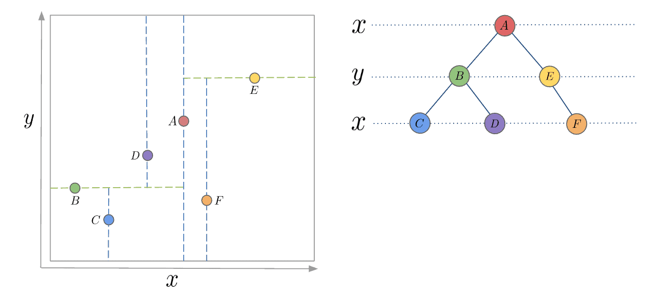
My FYP intrigues me into exploring acceleration of vector search. Based on my previous knowledge, in game / navigation, in order to speed up the search process, a common solution is to use K-D Trees, which recursively partition orthognal axies to construct a tree structure so that it only takes time complexity O(log n) to search, referring to Fig. 1.
However, even though partitioning sounds intuitive, it does not work well when the dimensions grows explosively into 256 or 1024, which will bring a long time to partition into all k dimensions. Therefore, I am going to break down a few techiniques that are used for speeding up ANN process step by step.
This article is going to mostly cover vector search parts so we do not discuss about inverted index and Learning-to-Rank.
Starting from K-NN
It is not a secret that K-Nearest Neighbors (K-NN) is the simplest and most naive nearest neighbor search algorithm.
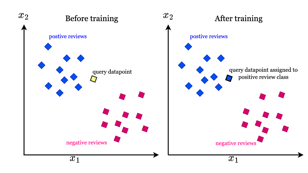
The principle of KNN algorithm is very simple: try to find the nearest neighbor of the query vector in the dataset. Usually these neighbors are belonged to a cluster so that it is able to put the query vector into specific class. This brutal algorithm’s time complexity is O(ND + Nlog(K)), where N denotes the number of vectors in the dataset and D denotes the dimension of the vectors, and Nlog(K) means to maintain the order of the candidate neighbors. Then KNN algorithm also can extend to find the nearest cluster to categorize each query, as shown in Fig. 2.
However, when the vector dimension explodes or the number of vectors vastly increases, K-NN algorithm reveals weakness in terms of its time complexity to inevitably calculate the euclidean distance for each and every vector in the dataset.
Anyway, I use Claude to generate a template for me to evaluate on ms-marco dataset, which you can find them appear in everywhere whenever it comes to searching, RAG or anything similar to information retrieval. Then I simulate K-NN algorithm by numpy through sorting euclidean distance for each queries. Then I calculate Recall, MRR and time cost taken by the algorithm.
import numpy as np
import time
from sentence_transformers import SentenceTransformer
from datasets import load_dataset
from tqdm import tqdm

print("Loading model...")
model = SentenceTransformer('sentence-transformers/msmarco-MiniLM-L-6-v3')

# Load MS MARCO dataset
print("\nLoading dataset...")
dataset = load_dataset('ms_marco', 'v1.1', split='train[:10000]')

# Extract queries and build qrels
queries = []
qrels = {}
corpus = {}

print("\nProcessing data...")
for idx, item in enumerate(tqdm(dataset, desc="Processing items")):
    # Check if there are answers
    if item['answers'] and len(item['answers']) > 0:
        query_text = item['query']

        # Extract relevant passages
        relevant_passages = []
        passages = item['passages']

        # Add all passages to corpus (v1.1 doesn't have passage_id, need to create our own)
        for i in range(len(passages['passage_text'])):
            ptext = passages['passage_text'][i]
            is_selected = passages['is_selected'][i]

            # Create unique passage ID using query_id and passage index
            pid = f"{item['query_id']}_{i}"

            # Add to corpus
            if pid not in corpus:
                corpus[pid] = ptext

            # If it's a relevant passage, record it
            if is_selected == 1:
                relevant_passages.append(pid)

        # Only keep queries with relevant passages
        if relevant_passages:
            queries.append(query_text)
            qrels[len(queries) - 1] = set(relevant_passages)

print(f"\n{'='*50}")
print(f"Data Statistics:")
print(f"{'='*50}")
print(f"Queries: {len(queries)}")
print(f"Corpus: {len(corpus)}")
print(f"Average relevant docs per query: {np.mean([len(v) for v in qrels.values()]):.2f}")
print(f"{'='*50}")

# Prepare for encoding
corpus_ids = list(corpus.keys())
corpus_texts = list(corpus.values())

print("\nEncoding corpus...")
corpus_embeddings = model.encode(
    corpus_texts,
    batch_size=128,
    show_progress_bar=True,
    convert_to_numpy=True
)

print("\nEncoding queries...")
query_embeddings = model.encode(
    queries,
    batch_size=128,
    show_progress_bar=True,
    convert_to_numpy=True
)

# Normalize for cosine similarity
print("\nNormalizing embeddings...")
corpus_embeddings = corpus_embeddings / np.linalg.norm(corpus_embeddings, axis=1, keepdims=True)
query_embeddings = query_embeddings / np.linalg.norm(query_embeddings, axis=1, keepdims=True)

# KNN search
def knn_search(query_vecs, corpus_vecs, k=10):
    """Efficient KNN search using numpy"""
    scores = np.dot(query_vecs, corpus_vecs.T)
    top_k_idx = np.argsort(scores, axis=1)[:, -k:][:, ::-1]
    top_k_scores = np.take_along_axis(scores, top_k_idx, axis=1)
    return top_k_scores, top_k_idx

print("\nPerforming retrieval...")
retrieval_start = time.time()
scores, indices = knn_search(query_embeddings, corpus_embeddings, k=10)
retrieval_time = time.time() - retrieval_start
print(f"Search completed in {retrieval_time:.4f} seconds")

# Evaluation
print("\nCalculating evaluation metrics...")
mrr = 0.0
recall_at_10 = 0.0
precision_at_10 = 0.0
valid_queries = 0

for q_idx in tqdm(range(len(queries)), desc="Evaluating"):
    if q_idx not in qrels:
        continue

    relevant = qrels[q_idx]
    retrieved = [corpus_ids[idx] for idx in indices[q_idx]]

    # Calculate MRR
    for rank, doc_id in enumerate(retrieved, 1):
        if doc_id in relevant:
            mrr += 1.0 / rank
            break

    # Calculate Recall@10
    hits = len(set(retrieved) & relevant)
    recall_at_10 += hits / len(relevant)

    # Calculate Precision@10
    precision_at_10 += hits / len(retrieved)

    valid_queries += 1

# Average metrics
mrr /= valid_queries
recall_at_10 /= valid_queries
precision_at_10 /= valid_queries

print(f"\n{'='*50}")
print(f"Evaluation Results:")
print(f"{'='*50}")
print(f"Number of evaluated queries: {valid_queries}")
print(f"MRR@10:        {mrr:.4f}")
print(f"Recall@10:     {recall_at_10:.4f}")
print(f"Precision@10:  {precision_at_10:.4f}")
print(f"{'='*50}")
Results
Loading dataset...

Processing data...
Processing items: 100%|████████████████████████████████████████████████████████████████████████████████████████████████████████████████████████████████████████████████████████████████████████████| 10000/10000 [00:00<00:00, 13605.77it/s]

==================================================
Data Statistics:
==================================================
Queries: 9690
Corpus: 80128
Average relevant docs per query: 1.12
==================================================

Encoding corpus...
Batches: 100%|████████████████████████████████████████████████████████████████████████████████████████████████████████████████████████████████████████████████████████████████████████████████████████████| 626/626 [00:39<00:00, 15.77it/s]

Encoding queries...
Batches: 100%|█████████████████████████████████████████████████████████████████████████████████████████████████████████████████████████████████████████████████████████████████████████████████████████████| 76/76 [00:00<00:00, 103.18it/s]

Normalizing embeddings...

Performing retrieval...
Search completed in 33.6314 seconds

Calculating evaluation metrics...
Evaluating: 100%|███████████████████████████████████████████████████████████████████████████████████████████████████████████████████████████████████████████████████████████████████████████████████| 9690/9690 [00:00<00:00, 132921.27it/s]

==================================================
Evaluation Results:
==================================================
Number of evaluated queries: 9690
MRR@10:        0.5874
Recall@10:     0.9541
Precision@10:  0.1057
==================================================
How does this work? Easy. To find the top-10 results for each query vector, we brutally search nearest 10 vectors in the whole corpus.
We can tell the result is not fast enough since it takes 33 seconds (which HNSW later will speed up so many times). Here, Recall@10 means how many of the top-10 results are relevant, MRR@10 means the average rank of the first relevant result in the top-10 results.
HNSW: Hierarchical Navigable Small World
A common thumb rule for speeding up querying is to pre-construct indexes or graphs beforehands, so that later it takes less efforts to compare each item.
Therefore, here goes our today’s first topic: HNSW (Hierarchical Navigable Small World). You probably have known this algorithm when using PostgreSQL vector searching or Faiss. Indeed, we can implement them by using Faiss but here we chose to implement by raw codes and break them down one by one.
Main Idea
HNSW is similar to Skip-list, as in that both of them are hierarchically splitting data points so that it enables the query to be only conducted in a smaller scope. For Skip-list, inserting, querying, deleting are all O(log n) and Redis uses Skip-list to store Key-Value pairs in memory, instead of red-black tree.
I have been told that the reason Redis uses Skip-list is because it is just simpler to implement. Not sure if it is true.
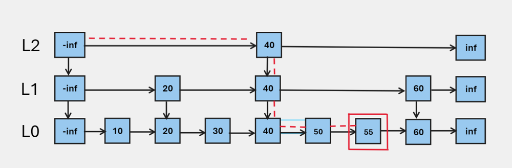
I will summarize the idea as Play it smart, not hard, since it does not go through EVERY item to find out the result. This is definitely a game changer for retrieval tasks. We also can tell that higher layer is always less dense than the layer below.
The way that HNSW stores hierarchical structure is to make a skip-list where the number of nodes in layer is always 1 / of the layer . And this will be guaranteed by the formula of randomness below:
where is a random number between 0 and 1. This $L% is calculated every time when there is a new vector inserting in HNSW graph.
Code Implemntation 1 - Initializing indexes
As mentioned above, we need to calculate the layer of the graph every time when there is a new vector inserting in HNSW graph.
def get_layer(self):
        return int(-np.log(np.random.random()) * self.mL)
This method makes sure that the probability of vectors are inserted into right places. You can see the effect by calling and outputing from this function. It will show most nodes are allocated in 0, some are in 1 then less are in 2 and etc.
There goes to our first function: search_in_one_layer, as the name suggests, it is used to search vector along with ef neighbors of entry_point in one layer of the graph.
It ends up returnning a List[Tuple[float, int]] where the first element is the distance and the second element is the index of the vector.
The index of vector and its actual matrix is saved in
self.corpus_vecs. And the graph of HNSW is indicated byself.graph.
Some initializations:
def __init__(self, corpus_vecs):
    self.entry_point = None
    self.corpus_vecs = corpus_vecs
    self.M = 16
    self.ef_construction = 200
    self.graph: List[dict[int, Set[int]]] = [] # the graph that saves NSW
    self.id = 0
    self.mL = 1 / np.log(self.M)
    def search_in_one_layer(self, vector, entry_point: Set[int], ef=1, L=0) -> List[Tuple[float, int]]:
        # search in Lth layer of the graph
        # return: for layer L, whats the neighbor of vectors 【Float, Int]
        # ef: number of neighbors to consider
        # find the nearest distance of neighbors
        visited = set(entry_point)
        candidates = [] #min heap
        results = [] #max heap, top of heap maintains the furtherest vector to be kicked out by pop

        for ep in entry_point: # get distance between query vector to entry points
            dist = self.get_distance(vector, self.corpus_vecs[ep])
            heapq.heappush(candidates, (dist, ep))
            heapq.heappush(results, (-dist, ep))

        while candidates:
            dist_c, c = heapq.heappop(candidates)
            dist_further = -results[0][0]
            if dist_c > dist_further and len(results) >=ef: # prune
                break

            neighbors = self.graph[L].get(c, set()) # the Lth layer to get c's neighbors

            for n in neighbors: # only search in neighbors of entry points
                if n not in visited:
                    visited.add(n)
                    dist = self.get_distance(vector, self.corpus_vecs[n])
                    if len(results) < ef or dist < -results[0][0]:
                        heapq.heappush(candidates, (dist, n))
                        heapq.heappush(results, (-dist, n))
                        if len(results) > ef:
                            heapq.heappop(results)
        result_sorted = sorted([(-d,n) for d,n in results])
        return result_sorted
Why keeping minimum heap and maximum heap at the same time? candidates is a min heap that help select the top-ef nearest neighbors, while results is used when requiring to kick out some vectors.
Since we kick out vectors by the furtherest distance, we use maximum heap to maintain the furtherest vector to be kicked out by pop.
select_neighbors_heuristic is supposed to be herutistic but this blog tend to follow minimalist implementation. So it simply sorted the distance and just get the top-M neighbors.
def select_neighbors_heuristic(self, candidates: List[Tuple[float, int]], M: int) -> Set[int]:
    """Select M neighbors using a heuristic to maintain graph connectivity"""
    if len(candidates) <= M:
        return {node_id for _, node_id in candidates}

    # Sort by distance (ascending)
    candidates = sorted(candidates)
    selected = set()

    for dist, node_id in candidates:
        if len(selected) >= M:
            break
        selected.add(node_id)

    return selected
Apetizers are ready, let’s move to main course: vector insertion.
The philosophy of inserting a vector can be described into two situations:
- When there is a first vector into HNSW, by the time HNSW has not yet got any levels, we will append the number of
level_currentlevels into graph variables, which is initiated fromget_layerfunction. - When it comes to new vectors, it searches through top layers down to the current layer + 1, to greedy search the entrypoint for the
nextlayer.
Why would using a greedy search for such a hassle situation? Because entry point passed from parameter is usually the toppest layer of vector, which you can still refer back to the Skip-list illustration.
Every time going down one layer, it would be hopping from the previous layer’s entry point to the next layer’s entry point. If we choose the same vector, it is no use because we already know the current vector is not the answer we want otherwise we should have stopped it here.
This is just a simple trick that sets ef as 1 here to just get the nearest neighbor as next entry point.
    def insert(self, query_vec):
        node_id = self.id
        self.id += 1
        level_current = self.get_layer() # get the level for this vector

        # Initialize graph layers if needed
        while len(self.graph) <= level_current:
            self.graph.append({})

        # First node - just add it
        if node_id == 0:
            self.entry_point = node_id
            for l in range(level_current + 1):
                self.graph[l][node_id] = set()
            return

        # Search phase 1: find entry points from top to target layer
        ep = {self.entry_point}
        max_level = len(self.graph) - 1

        # Navigate from top layer down to level_current+1
        for l in range(max_level, level_current, -1):
            results = self.search_in_one_layer(query_vec, ep, ef=1, L=l)
            ep = {results[0][1]} if results else ep

        # Search phase 2: find neighbors and insert at each layer from level_current down to 0
        for l in range(level_current, -1, -1):
            # Find ef_construction nearest neighbors at this layer
            results = self.search_in_one_layer(query_vec, ep, ef=self.ef_construction, L=l)

            # Select M neighbors for this layer
            M = self.M if l > 0 else self.M * 2  # Layer 0 has more connections
            neighbors = self.select_neighbors_heuristic(results, M)

            # Add bidirectional links
            if node_id not in self.graph[l]:
                self.graph[l][node_id] = set()

            for neighbor_id in neighbors:
                # Add edge from new node to neighbor
                self.graph[l][node_id].add(neighbor_id)

                # Add edge from neighbor to new node
                if neighbor_id not in self.graph[l]:
                    self.graph[l][neighbor_id] = set()
                self.graph[l][neighbor_id].add(node_id)

            # Update entry points for next layer
            ep = neighbors

        # Update entry point if new node is at a higher level
        if level_current > max_level:
            self.entry_point = node_id
Here we search through one layer and get neighbors from it. We select M neighbors to connect them within this layer.
So when constructing the edge between vectors, it means insert into graph. If this layer only has one vector, then only connects to this vector. But entrypoint is always added to result first as written in the beginning ofsearch_in_one_layer function.
            # Find ef_construction nearest neighbors at this layer
            results = self.search_in_one_layer(query_vec, ep, ef=self.ef_construction, L=l)

            # Select M neighbors for this layer
            M = self.M if l > 0 else self.M * 2  # Layer 0 has more connections
            neighbors = self.select_neighbors_heuristic(results, M)

            # Add bidirectional links
            if node_id not in self.graph[l]:
                self.graph[l][node_id] = set()
Implementation 2: Searching
After constructing indexes, then we go to search within HNSW graph.
Same as index insertion and Skip-list, we search vectors from top to down, and it is an approximate search, which means it will lose some accuracy since it is always approximate.
Searching is rather simpler than insertion: We also adopt greedy search to explore each layers’ entry points.
When it comes to Layer 0, where all nodes exist, we use these entry points to search fo ef nearest neighbors.
Then the final results are returned.
def search(self, query_vec, k=10, ef=None):
        """Search for k nearest neighbors
        Args:
            query_vec: query vector (already normalized)
            k: number of nearest neighbors to return
            ef: size of the dynamic candidate list (default: max(ef_construction, k))
        Returns:
            List of (distance, node_id) tuples
        """
        if ef is None:
            ef = max(self.ef_construction, k)

        if self.entry_point is None:
            return []

        # Start from entry point at the top layer
        ep = {self.entry_point}
        max_level = len(self.graph) - 1

        # Phase 1: Navigate from top to layer 1
        for l in range(max_level, 0, -1):
            results = self.search_in_one_layer(query_vec, ep, ef=1, L=l)
            ep = {results[0][1]} if results else ep

        # Phase 2: Search at layer 0 with ef candidates
        results = self.search_in_one_layer(query_vec, ep, ef=ef, L=0)

        # Return top k results
        return results[:k]
You might have noticed that
entry_pointeach time we used is based on the toppest layer of vector that has been inserted last time.
Speeding up by changing the way of distance calculation
Honestly in the beginning, to query vectors without optimization is so degraded that it almost kept the same speed as K-NN. This also blew my mind because theoretically it should be much faster. Then One of most throttling part is actually my distance calculation method.
In my previous implementation, get_distance function was always called to directly calculate the euclidean distance between two vectors.
def get_distance(v1, v2):
    return np.linalg.norm(v1 - v2)
But this is very slow since it compares each row and column of the matrix. A simple yet effective way to speed up is to normalize all vectors first, and then use cosine similarity to calculate the distance.
def get_distance(v1, v2):
    return -np.dot(v1, v2)
Negativity is to make sure the larger the distance, the smaller the similarity, matching the theroem of minimum heap to find the top-k elements.
Speeding up by pruning / early-quit when inserting
This speeds up querying 2X in my case. I did not write this part in insertion because I did not want to complex the process.
In HNSW, it’s crucial to maintain a maximum degree (M) for each node to ensure the graph remains a “small world” network with logarithmic search complexity. If a node has too many edges, the search becomes inefficient. Therefore, when we add a back-link to a neighbor, we must check if that neighbor now has > M connections. If so, we re-evaluate all its connections and keep only the best M ones using the heuristic.
So after adding an edge into graph, we need to have a check:
if len(self.graph[l][neighbor_id]) > M:
    # Collect all existing connections of this neighbor
    current_connections = list(self.graph[l][neighbor_id])

    # Calculate distances from these connections to the neighbor_id
    conn_candidates = []
    neighbor_vec = self.corpus_vecs[neighbor_id]

    # Note: For simplicity, we calculate distances one by one.
    # In a production environment, vectorized calculation would be more efficient.
    for conn_id in current_connections:
        dist = self.get_distance(neighbor_vec, self.corpus_vecs[conn_id])
        conn_candidates.append((dist, conn_id))

    # Re-execute heuristic selection to retain only the best M connections
    kept_neighbors = self.select_neighbors_heuristic(conn_candidates, M)

    # Update the graph structure
    self.graph[l][neighbor_id] = kept_neighbors
Final Result
Loading model...

Loading dataset...

Processing data...
Processing items: 100%|█████████████████████████████████████████████████████████████████████████████████████| 10000/10000 [00:00<00:00, 22211.02it/s]

==================================================
Data Statistics:
==================================================
Queries: 9690
Corpus: 80128
Average relevant docs per query: 1.12
==================================================

Encoding corpus...
Batches: 100%|█████████████████████████████████████████████████████████████████████████████████████████████████████| 626/626 [00:36<00:00, 17.05it/s]

Encoding queries...
Batches: 100%|██████████████████████████████████████████████████████████████████████████████████████████████████████| 76/76 [00:00<00:00, 117.31it/s]

Normalizing embeddings...

Performing retrieval...
Building HNSW index...
Inserting vectors: 100%|██████████████████████████████████████████████████████████████████████████████████████| 80128/80128 [05:26<00:00, 245.23it/s]
HNSW index built with 80128 vectors

Searching queries...
Searching: 100%|███████████████████████████████████████████████████████████████████████████████████████████████| 9690/9690 [00:05<00:00, 1728.07it/s]
Search completed in 332.3713 seconds

Calculating evaluation metrics...
Evaluating: 100%|████████████████████████████████████████████████████████████████████████████████████████████| 9690/9690 [00:00<00:00, 296768.96it/s]

==================================================
Evaluation Results:
==================================================
Number of evaluated queries: 9690
MRR@10:        0.4968
Recall@10:     0.8122
Precision@10:  0.0902
==================================================
Querying is ultimately fast: within 5 seconds, it finishes where the BM25 K-NN search has to take 33 seconds to achieve.
But inserting indexes takes over 4 minutes, which is the trade-off of using this method. The truth is in real-world scenario, what we always care is online real-time results instead of the offline one.
Experimental Setup
All experiments are conducted on RTX 2080 ti, Intel Core i5-12450H, 16GB RAM, Manjaro. We use python=3.10 and all latest library by the time of writing.
For the references
Then following searching, Elastic search uses HNSW algorithm